
15.8. Analysis of Closed Hashing
15.8.1. Analysis of Closed Hashing
How efficient is hashing? We can measure hashing performance in terms of the number of record accesses required when performing an operation. The primary operations of concern are insertion, deletion, and search. It is useful to distinguish between successful and unsuccessful searches. Before a record can be deleted, it must be found. Thus, the number of accesses required to delete a record is equivalent to the number required to successfully search for it. To insert a record, an empty slot along the record’s probe sequence must be found. This is equivalent to an unsuccessful search for the record (recall that a successful search for the record during insertion should generate an error because two records with the same key are not allowed to be stored in the table).
When the hash table is empty, the first record inserted will always find its home position free. Thus, it will require only one record access to find a free slot. If all records are stored in their home positions, then successful searches will also require only one record access. As the table begins to fill up, the probability that a record can be inserted into its home position decreases. If a record hashes to an occupied slot, then the collision resolution policy must locate another slot in which to store it. Finding records not stored in their home position also requires additional record accesses as the record is searched for along its probe sequence. As the table fills up, more and more records are likely to be located ever further from their home positions.
From this discussion, we see that the expected cost of hashing is a function of how full the table is. Define the load factor for the table as \(\alpha = N/M\), where \(N\) is the number of records currently in the table.
An estimate of the expected cost for an insertion (or an unsuccessful search) can be derived analytically as a function of \(\alpha\) in the case where we assume that the probe sequence follows a random permutation of the slots in the hash table. Assuming that every slot in the table has equal probability of being the home slot for the next record, the probability of finding the home position occupied is \(\alpha\). The probability of finding both the home position occupied and the next slot on the probe sequence occupied is \((N(N-1))/(M(M-1))\). The probability of \(i\) collisions is \((N(N-1) ... (N-i+1))/(M(M-1) ... (M-i+1))\). If \(N\) and \(M\) are large, then this is approximately \((N/M)^i\). The expected number of probes is one plus the sum over \(i >= 1\) of the probability of \(i\) collisions, which is approximately
The cost for a successful search (or a deletion) has the same cost as originally inserting that record. However, the expected value for the insertion cost depends on the value of \(\alpha\) not at the time of deletion, but rather at the time of the original insertion. We can derive an estimate of this cost (essentially an average over all the insertion costs) by integrating from 0 to the current value of \(\alpha\), yielding a result of \((1/\alpha) \log_e 1/(1-\alpha).\)
It is important to realize that these equations represent the expected cost for operations when using the unrealistic assumption that the probe sequence is based on a random permutation of the slots in the hash table. We thereby avoid all the expense that results from a less-than-perfect collision resolution policy. Thus, these costs are lower-bound estimates in the average case. The true average cost under linear probing is \(.5(1 + 1/(1-\alpha)^2)\) for insertions or unsuccessful searches and \(.5(1 + 1/(1-\alpha))\) for deletions or successful searches.
Todo
- type: Text
Where did that last claim about the linear probing cost come from?
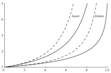
Figure 15.8.1: A plot showing the growth rate of the cost for insertion and deletion into a hash table as the load factor increases.
Figure 15.8.1 shows how the expected number of record accesses grows as \(\alpha\) grows. The horizontal axis is the value for \(\alpha\) , the vertical axis is the expected number of accesses to the hash table. Solid lines show the cost for “random” probing (a theoretical lower bound on the cost), while dashed lines show the cost for linear probing (a relatively poor collision resolution strategy). The two leftmost lines show the cost for insertion (equivalently, unsuccessful search); the two rightmost lines show the cost for deletion (equivalently, successful search).
From the figure, you should see that the cost for hashing when the table is not too full is typically close to one record access. This is extraordinarily efficient, much better than binary search which requires \(\log n\) record accesses. As \(\alpha\) increases, so does the expected cost. For small values of \(\alpha\), the expected cost is low. It remains below two until the hash table is about half full. When the table is nearly empty, adding a new record to the table does not increase the cost of future search operations by much. However, the additional search cost caused by each additional insertion increases rapidly once the table becomes half full. Based on this analysis, the rule of thumb is to design a hashing system so that the hash table never gets above about half full, because beyond that point performance will degrade rapidly. This requires that the implementor have some idea of how many records are likely to be in the table at maximum loading, and select the table size accordingly. The goal should be to make the table small enough so that it does not waste a lot of space on the one hand, while making it big enough to keep performance good on the other.