
15.7. Other Spatial Data Structures
The differences between the kd tree and the PR quadtree illustrate many of the design choices encountered when creating spatial data structures. The kd tree provides an object-space decomposition of the region, while the PR quadtree provides a key-space decomposition (thus, it is a trie). The kd tree stores records at all nodes, while the PR quadtree stores records only at the leaf nodes. Finally, the two trees have different structures. The kd tree is a binary tree (and need not be full), while the PR quadtree is a full tree with \(2^d\) branches (in the two-dimensional case, \(2^2 = 4\)). Consider the extension of this concept to three dimensions. A kd tree for three dimensions would alternate the discriminator through the \(x\), \(y\), and \(z\) dimensions. The three-dimensional equivalent of the PR quadtree would be a tree with \(2^3\) or eight branches. Such a tree is called an octree.
Consider the differences between the PR quadtree and the Bintree. Both use object-space decomposition, and so both are tries. But they are different in the the PR quadtree splits in all dimensions at once, while the Bintree rotates through its dimensions, splitting one at a time.
Alternatively, we can use a four-way decomposition of space centered on the data points. The tree resulting from such a decomposition is called a point quadtree. This could be viewed as the object-space decomposition analog of the PR quadtree. Or it could be viewed as a variation on the kd-tree that splits all dimensions at once. An example point quadtree is shown in Figure 15.7.1.
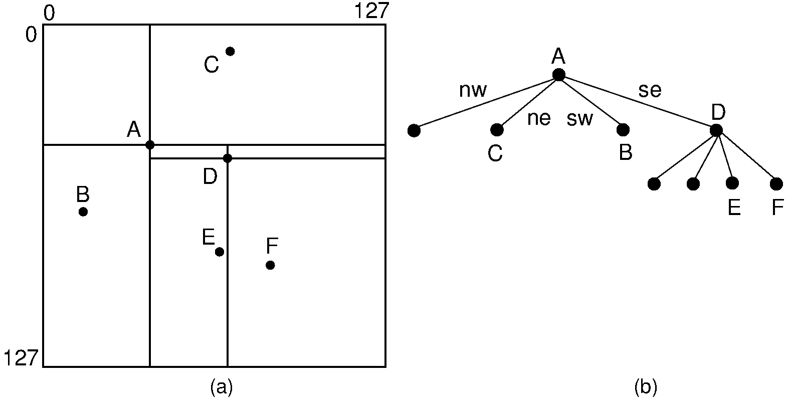
Figure 15.7.1: An example of the point quadtree, a 4-ary tree using object-space decomposition. Compare this with the PR quadtree of Figure 15.4.1.
Our discussion of spatial data structures for storing points has barely scratched the surface of the field of spatial data structures. Dozens of distinct spatial data structures have been invented, many with variations and alternate implementations. Spatial data structures exist for storing many forms of spatial data other than points. The most important distinctions between are the tree structure (binary or not, regular decompositions or not) and the decomposition rule used to decide when the data contained within a region is so complex that the region must be subdivided.
One such spatial data structure is the Region Quadtree for storing images where the pixel values tend to be blocky, such as a map of the countries of the world. The region quadtree uses a four-way regular decomposition scheme similar to the PR quadtree The decomposition rule is simply to divide any node containing pixels of more than one color or value.
Spatial data structures can also be used to store line object, rectangle object, or objects of arbitrary shape (such as polygons in two dimensions or polyhedra in three dimensions). A simple, yet effective, data structure for storing rectangles or arbitrary polygonal shapes can be derived from the PR quadtree. Pick a threshold value \(c\), and subdivide any region into four quadrants if it contains more than \(c\) objects. A special case must be dealt with when more than \(c\) objects intersect.
Some of the most interesting developments in spatial data structures have to do with adapting them for disk-based applications. However, all such disk-based implementations boil down to storing the spatial data structure within some variant on either B-trees or hashing.