
15.5. KD Trees
15.5.1. KD Trees
The kd tree is a modification to the BST that allows for efficient processing of multi-dimensional search keys. The kd tree differs from the BST in that each level of the kd tree makes branching decisions based on a particular search key associated with that level, called the discriminator. In principle, the kd tree could be used to unify key searching across any arbitrary set of keys such as name and zipcode. But in practice, it is nearly always used to support search on multi-dimensional coordinates, such as locations in 2D or 3D space. We define the discriminator at level \(i\) to be \(i\) mod \(k\) for \(k\) dimensions. For example, assume that we store data organized by \(xy\)-coordinates. In this case, \(k\) is 2 (there are two coordinates), with the \(x\)-coordinate field arbitrarily designated key 0, and the \(y\)-coordinate field designated key 1. At each level, the discriminator alternates between \(x\) and \(y\). Thus, a node \(N\) at level 0 (the root) would have in its left subtree only nodes whose \(x\) values are less than \(N_x\) (because \(x\) is search key 0, and \(0 \mod 2 = 0\)). The right subtree would contain nodes whose \(x\) values are greater than \(N_x\). A node \(M\) at level 1 would have in its left subtree only nodes whose \(y\) values are less than \(M_y\). There is no restriction on the relative values of \(M_x\) and the \(x\) values of \(M\) ‘s descendants, because branching decisions made at \(M\) are based solely on the \(y\) coordinate. Figure 15.5.1 shows an example of how a collection of two-dimensional points would be stored in a kd tree.
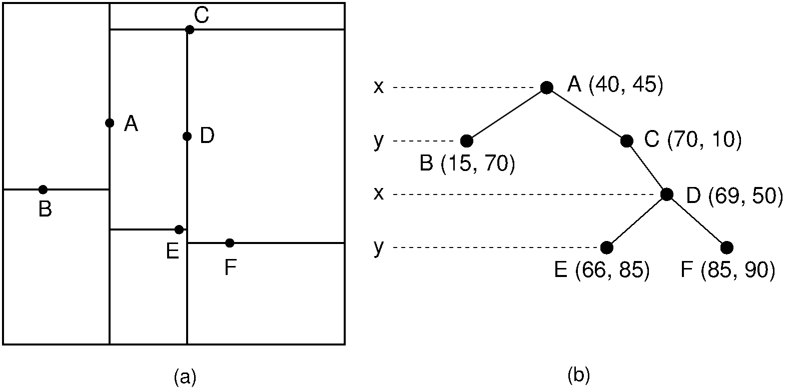
Figure 15.5.1: Example of a kd tree. (a) The kd tree decomposition for a \(128 \times 128\)-unit region containing seven data points. (b) The kd tree for the region of (a).
In Figure 15.5.1, the region containing the points is (arbitrarily) restricted to a \(128 \times 128\) square, and each internal node splits the search space. Each split is shown by a line, vertical for nodes with \(x\) discriminators and horizontal for nodes with \(y\) discriminators. The root node splits the space into two parts; its children further subdivide the space into smaller parts. The children’s split lines do not cross the root’s split line. Thus, each node in the kd tree helps to decompose the space into rectangles that show the extent of where nodes can fall in the various subtrees.
Searching a kd tree for the record with a specified xy-coordinate is like searching a BST, except that each level of the kd tree is associated with a particular discriminator.
private E findhelp(KDNode<E> rt, int[] key, int level) {
  if (rt == null) return null;
  E it = rt.element();
  int[] itkey = rt.key();
  if ((itkey[0] == key[0]) && (itkey[1] == key[1]))
    return rt.element();
  if (itkey[level] > key[level])
    return findhelp(rt.left(), key, (level+1)%D);
  else
    return findhelp(rt.right(), key, (level+1)%D);
}
Inserting a new node into the kd tree is similar to
BST insertion.
The kd tree search procedure is followed until a NULL pointer is
found, indicating the proper place to insert the new node.
Deleting a node from a kd tree is similar to deleting from a BST,
but slightly harder.
As with deleting from a BST, the first step is to find the node
(call it \(N\)) to be deleted.
It is then necessary to find a descendant of \(N\) which can be
used to replace \(N\) in the tree.
If \(N\) has no children, then \(N\) is replaced with a
NULL pointer.
Note that if \(N\) has one child that in turn has children, we
cannot simply assign \(N\)’s parent to point to \(N\)’s
child as would be done in the BST.
To do so would change the level of all nodes in the subtree, and thus
the discriminator used for a search would also change.
The result is that the subtree would no longer be a kd tree because a
node’s children might now violate the BST property for that
discriminator.
Similar to BST deletion, the record stored in \(N\) should
be replaced either by the record in \(N\)’s right subtree with
the least value of \(N\)’s discriminator, or by the record in
\(N\)’s left subtree with the greatest value for this
discriminator.
Assume that \(N\) was at an odd level and therefore \(y\) is
the discriminator.
\(N\) could then be replaced by the record in its right subtree
with the least \(y\) value (call it \(Y_{min}\)).
The problem is that \(Y_{min}\) is not necessarily the
leftmost node, as it would be in the BST.
A modified search procedure to find the least \(y\) value in the
left subtree must be used to find it instead.
The implementation for findmin is shown next.
A recursive call to the delete routine will then remove
\(Y_{min}\) from the tree.
Finally, \(Y_{min}\)’s record is substituted for the
record in node \(N\).
private KDNode<E>
findmin(KDNode<E> rt, int descrim, int level) {
  KDNode<E> temp1, temp2;
  int[] key1 = null;
  int[] key2 = null;
  if (rt == null) return null;
  temp1 = findmin(rt.left(), descrim, (level+1)%D);
  if (temp1 != null) key1 = temp1.key();
  if (descrim != level) {
    temp2 = findmin(rt.right(), descrim, (level+1)%D);
    if (temp2 != null) key2 = temp2.key();
    if ((temp1 == null) || ((temp2 != null) &&
                   (key1[descrim] > key2[descrim]))) {
      temp1 = temp2;
      key1 = key2;
    }
  } // Now, temp1 has the smaller value
  int[] rtkey = rt.key();
  if ((temp1 == null) || (key1[descrim] > rtkey[descrim]))
    return rt;
  else
    return temp1;
}
In findmin, on levels using the minimum value’s discriminator,
branching is to the left.
On other levels, both children’s subtrees must be visited.
Helper function min takes two nodes and a discriminator as
input, and returns the node with the smaller value in that
discriminator.
Note that we can replace the node to be deleted with the least-valued node from the right subtree only if the right subtree exists. If it does not, then a suitable replacement must be found in the left subtree. Unfortunately, it is not satisfactory to replace \(N\)’s record with the record having the greatest value for the discriminator in the left subtree, because this new value might be duplicated. If so, then we would have equal values for the discriminator in \(N\)’s left subtree, which violates the ordering rules for the kd tree. Fortunately, there is a simple solution to the problem. We first move the left subtree of node \(N\) to become the right subtree (i.e., we simply swap the values of \(N\)’s left and right child pointers). At this point, we proceed with the normal deletion process, replacing the record of \(N\) to be deleted with the record containing the least value of the discriminator from what is now \(N\)’s right subtree.
Assume that we want to print out a list of all records that are within a certain distance \(d\) of a given point \(P\). We will use Euclidean distance, that is, point \(P\) is defined to be within distance \(d\) of point \(N\) if \(\sqrt{(P_x - N_x)^2 + (P_y - N_y)^2} \leq d.\) [1]
If the search process reaches a node whose key value for the discriminator is more than \(d\) above the corresponding value in the search key, then it is not possible that any record in the right subtree can be within distance \(d\) of the search key because all key values in that dimension are always too great. Similarly, if the current node’s key value in the discriminator is \(d\) less than that for the search key value, then no record in the left subtree can be within the radius. In~such cases, the subtree in question need not be searched, potentially saving much time. In the average case, the number of nodes that must be visited during a range query is linear on the number of data records that fall within the query circle.
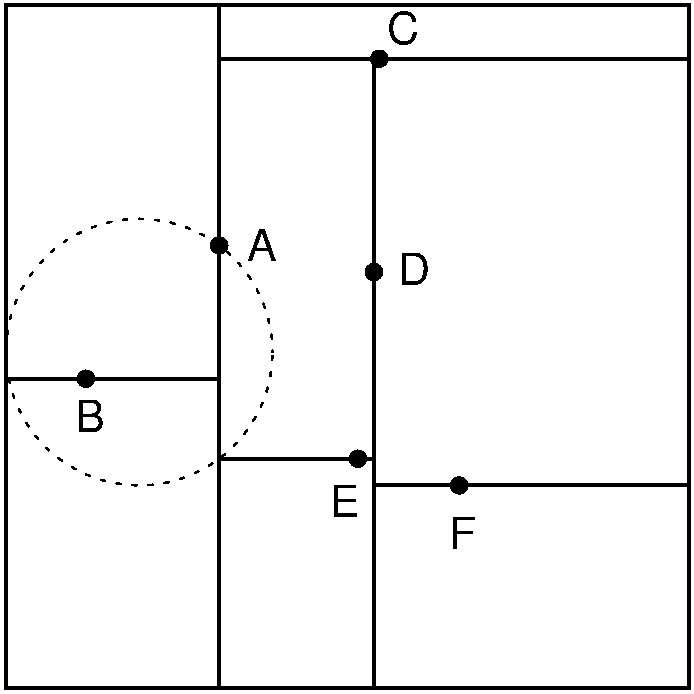
Figure 15.5.2: Searching in the kd tree of Figure 15.5.1. (a) The kd tree decomposition for a \(128 \times 128\)-unit region containing seven data points. (b) The kd tree for the region of (a).
Here is an implementation for the region search method.
private void rshelp(KDNode<E> rt, int[] point,
                    int radius, int lev) {
  if (rt == null) return;
  int[] rtkey = rt.key();
  if (InCircle(point, radius, rtkey))
    System.out.println(rt.element());
  if (rtkey[lev] > (point[lev] - radius))
    rshelp(rt.left(), point, radius, (lev+1)%D);
  if (rtkey[lev] < (point[lev] + radius))
    rshelp(rt.right(), point, radius, (lev+1)%D);
}
When a node is visited, function InCircle is used to
check the Euclidean distance between the node’s record and the query
point.
It is not enough to simply check that the differences between the
\(x\)- and \(y\)-coordinates are each less than the query
distances because the the record could still be outside the search
circle, as illustrated by Figure 15.5.3.
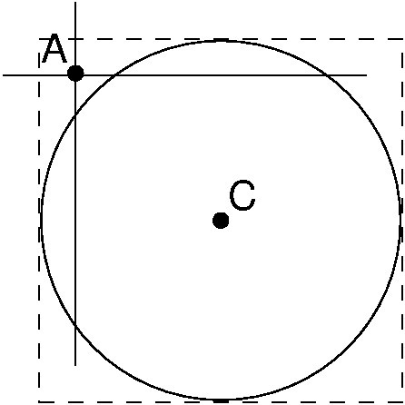
Figure 15.5.3: Function InCircle must check the Euclidean distance
between a record and the query point.
It is possible for a record \(A\) to have \(x\)- and
\(y\)-coordinates each within the query distance of the query
point \(C\), yet have \(A\) itself lie outside the query
circle.
Here is a visualization of building a kd-tree.