
26.3. The Splay Tree
Like the AVL tree, the splay tree is not actually a distinct data structure, but rather reimplements the BST insert, delete, and search methods to improve the performance of a BST. The goal of these revised methods is to provide guarantees on the time required by a series of operations, thereby avoiding the worst-case linear time behavior of standard BST operations. No single operation in the splay tree is guaranteed to be efficient. Instead, the splay tree access rules guarantee that a series of \(m\) operations will take \(O(m log n)\) time for a tree of \(n\) nodes whenever \(m \geq n\). Thus, a single insert or search operation could take \(O(n)\) time. However, \(m\) such operations are guaranteed to require a total of \(O(m \log n)\) time, for an average cost of \(O(\log n)\) per access operation. This is a desirable performance guarantee for any search-tree structure.
Unlike the AVL tree, the splay tree is not guaranteed to be height balanced. What is guaranteed is that the total cost of the entire series of accesses will be cheap. Ultimately, it is the cost of the series of operations that matters, not whether the tree is balanced. Maintaining balance is really done only for the sake of reaching this time efficiency goal.
The splay tree access functions operate in a manner reminiscent of the move-to-front rule for self-organizing lists, and of the path compression technique for managing a series of Union/Find operations. These access functions tend to make the tree more balanced, but an individual access will not necessarily result in a more balanced tree.
Whenever a node \(S\) is accessed (e.g., when \(S\) is inserted, deleted, or is the goal of a search), the splay tree performs a process called splaying. Splaying moves \(S\) to the root of the BST. When \(S\) is being deleted, splaying moves the parent of \(S\) to the root. As in the AVL tree, a splay of node \(S\) consists of a series of rotations. A rotation moves \(S\) higher in the tree by adjusting its position with respect to its parent and grandparent. A side effect of the rotations is a tendency to balance the tree. There are three types of rotation.
A single rotation is performed only if \(S\) is a child of the root node. The single rotation is illustrated by Figure 26.3.1. It basically switches \(S\) with its parent in a way that retains the BST property. While Figure 26.3.1 is slightly different from Figure 26.2.2, in fact the splay tree single rotation is identical to the AVL tree single rotation.
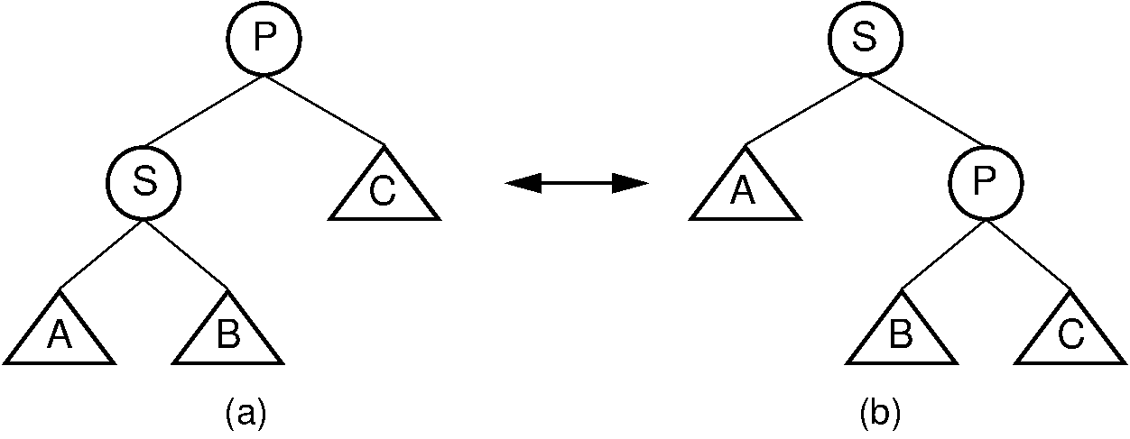
Figure 26.3.1: Splay tree single rotation. This rotation takes place only when the node being splayed is a child of the root. Here, node \(S\) is promoted to the root, rotating with node \(P\). Because the value of \(S\) is less than the value of \(P\), \(P\) must become \(S\) ‘s right child. The positions of subtrees \(A\), \(B\), and ;math:C are altered as appropriate to maintain the BST property, but the contents of these subtrees remains unchanged. (a) The original tree with \(P\) as the parent. (b) The tree after a rotation takes place. Performing a single rotation a second time will return the tree to its original shape. Equivalently, if (b) is the initial configuration of the tree (i.e., \(S\) is at the root and \(P\) is its right child), then (a) shows the result of a single rotation to splay \(P\) to the root.
Unlike the AVL tree, the splay tree requires two types of double rotation. Double rotations involve \(S\), its parent (call it \(P\)), and \(S\) ‘s grandparent (call it \(G\)). The effect of a double rotation is to move \(S\) up two levels in the tree.
The first double rotation is called a \(zigzag rotation\). It takes place when either of the following two conditions are met:
\(S\) is the left child of \(P\), and \(P\) is the right child of \(G\).
\(S\) is the right child of \(P\), and \(P\) is the left child of \(G\).
In other words, a zigzag rotation is used when \(G\), \(P\), and \(S\) form a zigzag. The zigzag rotation is illustrated by Figure 26.3.2.
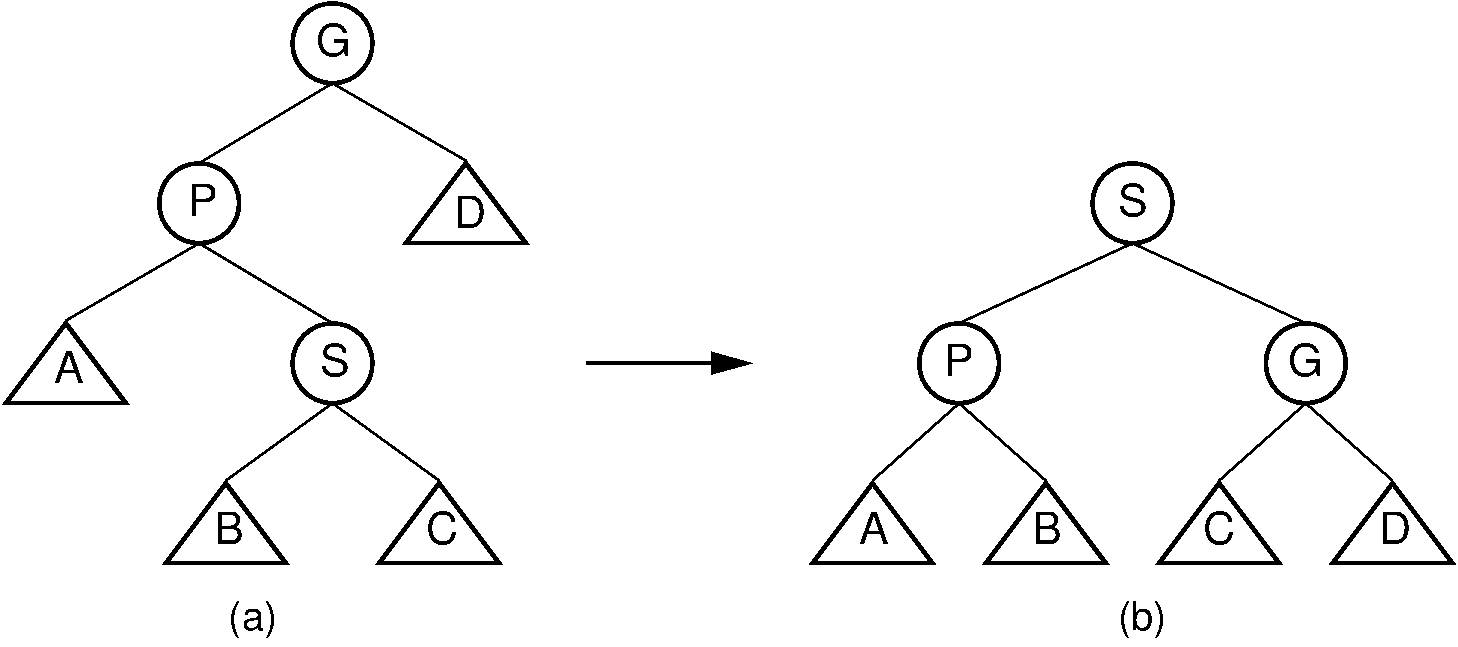
Figure 26.3.2: Splay tree zigzag rotation. (a) The original tree with \(S\), \(P\), and \(G\) in zigzag formation. (b) The tree after the rotation takes place. The positions of subtrees \(A\), \(B\), \(C\), and \(D\) are altered as appropriate to maintain the BST property.
The other double rotation is known as a zigzig rotation. A zigzig rotation takes place when either of the following two conditions are met:
\(S\) is the left child of \(P\), which is in turn the left child of \(G\).
\(S\) is the right child of \(P\), which is in turn the right child of \(G\).
Thus, a zigzig rotation takes place in those situations where a zigzag rotation is not appropriate. The zigzig rotation is illustrated by Figure 26.3.3. While Figure 26.3.3 appears somewhat different from Figure 26.2.3, in fact the zigzig rotation is identical to the AVL tree double rotation.
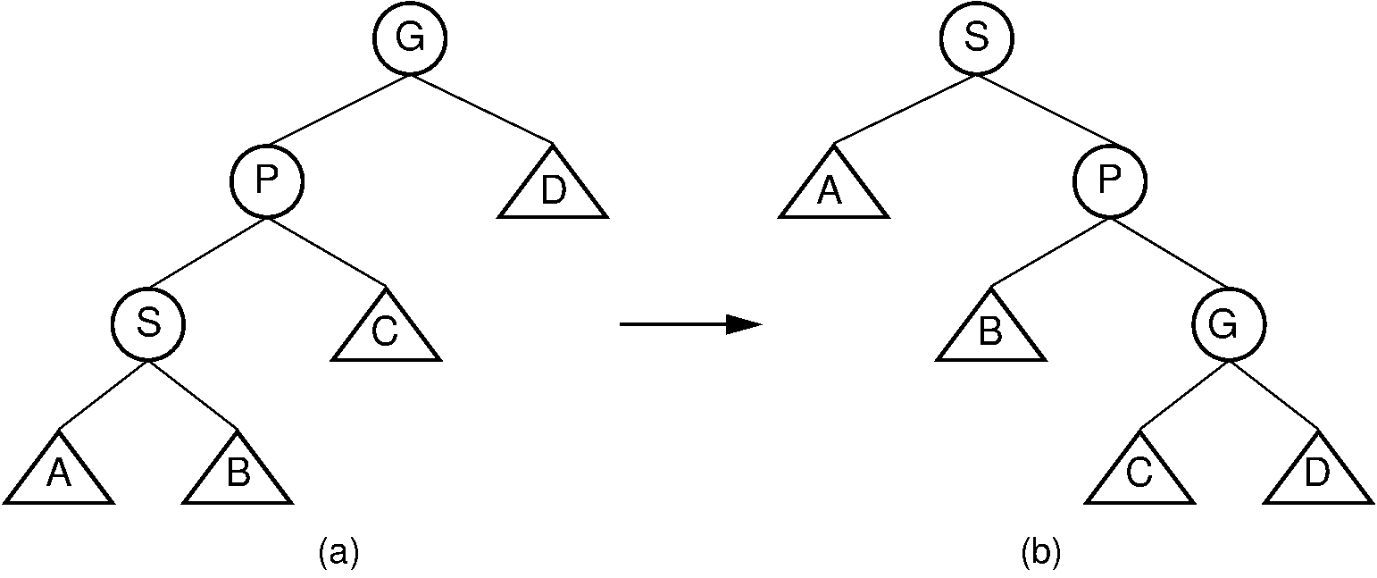
Figure 26.3.3: Splay tree zigzig rotation. (a) The original tree with \(S\), \(P\), and \(G\) in zigzig formation. (b) The tree after the rotation takes place. The positions of subtrees \(A\), \(B\), \(C\), and \(D\) are altered as appropriate to maintain the BST property.
Note that zigzag rotations tend to make the tree more balanced, because they bring subtrees \(B\) and \(C\) up one level while moving subtree \(D\) down one level. The result is often a reduction of the tree’s height by one. Zigzig promotions and single rotations do not typically reduce the height of the tree; they merely bring the newly accessed record toward the root.
Splaying node \(S\) involves a series of double rotations until \(S\) reaches either the root or the child of the root. Then, if necessary, a single rotation makes \(S\) the root. This process tends to re-balance the tree. Regardless of balance, splaying will make frequently accessed nodes stay near the top of the tree, resulting in reduced access cost. Proof that the splay tree meets the guarantee of \(O(m \log n)\) is beyond the scope of our study.
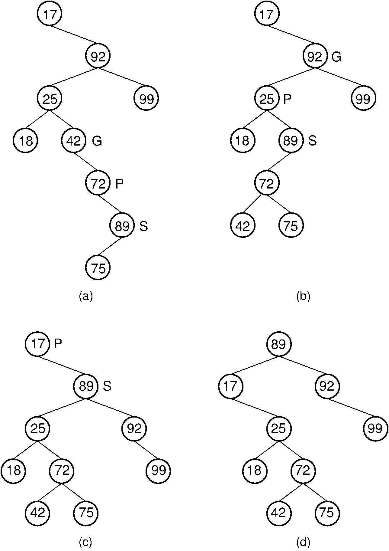
Figure 26.3.4: Example of splaying after performing a search in a splay tree. After finding the node with key value 89, that node is splayed to the root by performing three rotations. (a) The original splay tree. (b) The result of performing a zigzig rotation on the node with key value 89 in the tree of (a). (c) The result of performing a zigzag rotation on the node with key value 89 in the tree of (b). (d) The result of performing a single rotation on the node with key value 89 in the tree of (c). If the search had been for 91, the search would have been unsuccessful with the node storing key value 89 being that last one visited. In that case, the same splay operations would take place.