27.9.1.1. Introduction¶

We now tackle the problem of devising an implementation for general trees that allows efficient processing for all member functions of the ADTs of Module <GenTreeIntro>. This section presents several approaches to implementing general trees. Each implementation yields advantages and disadvantages in the amount of space required to store a node and the relative ease with which key operations can be performed. General tree implementations should place no restriction on how many children a node may have. In some applications, once a node is created the number of children never changes. In such cases, a fixed amount of space can be allocated for the node when it is created, based on the number of children for the node. Matters become more complicated if children can be added to or deleted from a node, requiring that the node’s space allocation be adjusted accordingly.

27.9.1.2. List of Children¶

Our first attempt to create a general tree implementation is called the “list of children” implementation for general trees. It simply stores with each internal node a linked list of its children. This is illustrated by Figure 27.9.1.

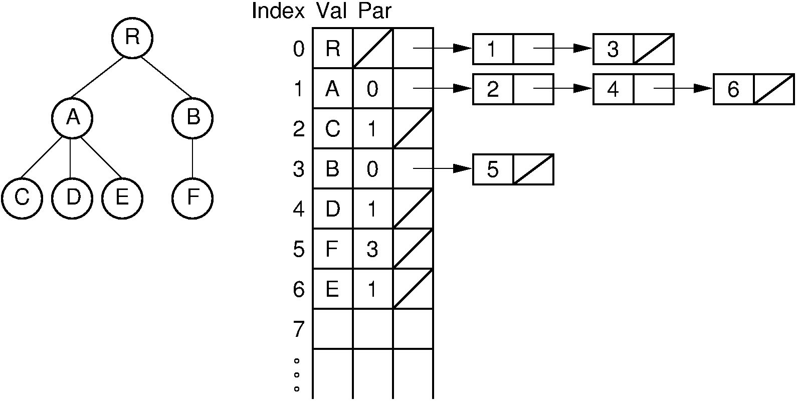
Figure 27.9.1: The “list of children” implementation for general trees. The column of numbers to the left of the node array labels the array indices. The column labeled “Val” stores node values. The column labeled “Par” stores indices (or pointers) to the parents. The last column stores pointers to the linked list of children for each internal node. Each element of the linked list stores a pointer to one of the node’s children (shown as the array index of the target node).¶

The “list of children” implementation stores the tree nodes in an array. Each node contains a value, a pointer (or index) to its parent, and a pointer to a linked list of the node’s children, stored in order from left to right. Each linked list element contains a pointer to one child. Thus, the leftmost child of a node can be found directly because it is the first element in the linked list. However, to find the right sibling for a node is more difficult. Consider the case of a node \(M\) and its parent \(P\). To find \(M\) ‘s right sibling, we must move down the child list of \(P\) until the linked list element storing the pointer to \(M\) has been found. Going one step further takes us to the linked list element that stores a pointer to \(M\) ‘sright sibling. Thus, in the worst case, to find \(M\) ‘s right sibling requires that all children of \(M\) ‘s parent be searched.

Combining trees using this representation is difficult if each tree is stored in a separate node array. If the nodes of both trees are stored in a single node array, then adding tree \(\mathbf{T}\) as a subtree of node \(R\) is done by simply adding the root of \(\mathbf{T}\) to \(R\) ‘s list of children.

27.9.1.3. The Left-Child/Right-Sibling Implementation¶

With the “list of children” implementation, it is difficult to access a node’s right sibling. Figure 27.9.2 presents an improvement. Here, each node stores its value and pointers to its parent, leftmost child, and right sibling. Thus, each of the basic ADT operations can be implemented by reading a value directly from the node. If two trees are stored within the same node array, then adding one as the subtree of the other simply requires setting three pointers. Combining trees in this way is illustrated by Figure 27.9.3. This implementation is more space efficient than the “list of children” implementation, and each node requires a fixed amount of space in the node array.

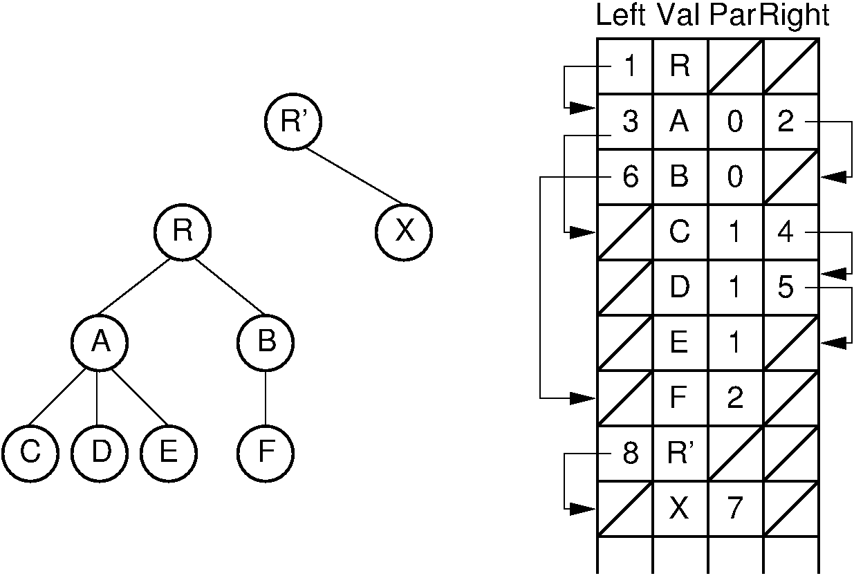
Figure 27.9.2: The “left-child/right-sibling” implementation.¶

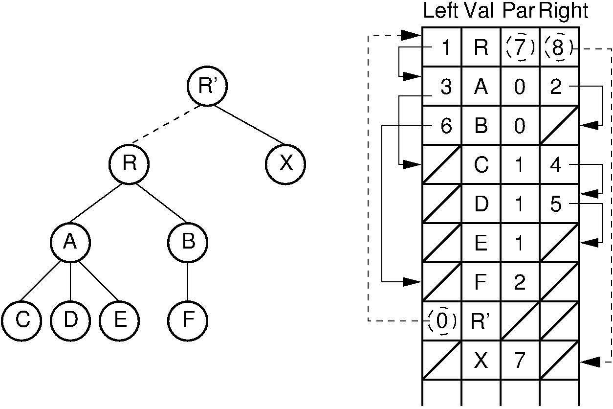
Figure 27.9.3: Combining two trees that use the “left-child/right-sibling” implementation. The subtree rooted at \(R\) in Figure 27.9.2 now becomes the first child of \(R'\). Three pointers are adjusted in the node array: The left-child field of \(R'\) now points to node \(R\), while the right-sibling field for \(R\) points to node \(X\). The parent field of node \(R\) points to node \(R'\).¶

27.9.1.4. Dynamic Node Implementations¶

The two general tree implementations just described use an array to store the collection of nodes. In contrast, our standard implementation for binary trees stores each node as a separate dynamic object containing its value and pointers to its two children. Unfortunately, nodes of a general tree can have any number of children, and this number may change during the life of the node. A general tree node implementation must support these properties. One solution is simply to limit the number of children permitted for any node and allocate pointers for exactly that number of children. There are two major objections to this. First, it places an undesirable limit on the number of children, which makes certain trees unrepresentable by this implementation. Second, this might be extremely wasteful of space because most nodes will have far fewer children and thus leave some pointer positions empty.

The alternative is to allocate variable space for each node. There are two basic approaches. One is to allocate an array of child pointers as part of the node. In essence, each node stores an array-based list of child pointers. Figure 27.9.4 illustrates the concept. This approach assumes that the number of children is known when the node is created, which is true for some applications but not for others. It also works best if the number of children does not change. If the number of children does change (especially if it increases), then some special recovery mechanism must be provided to support a change in the size of the child pointer array. One possibility is to allocate a new node of the correct size from free store and return the old copy of the node to free store for later reuse. This works especially well in a language with built-in garbage collection such as Java. For example, assume that a node \(M\) initially has two children, and that space for two child pointers is allocated when \(M\) is created. If a third child is added to \(M\), space for a new node with three child pointers can be allocated, the contents of \(M\) is copied over to the new space, and the old space is then returned to free store. As an alternative to relying on the system’s garbage collector, a memory manager for variable size storage units can be implemented, as described in Chapter Memory Management. Another possibility is to use a collection of free lists, one for each array size, as described in Module <Freelist>. Note in Figure 27.9.4 that the current number of children for each node is stored explicitly in a size field. The child pointers are stored in an array with size elements.

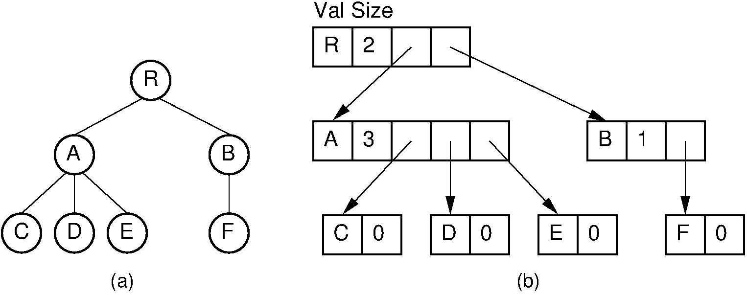
Figure 27.9.4: A dynamic general tree representation with fixed-size arrays for the child pointers. (a) The general tree. (b) The tree representation. For each node, the first field stores the node value while the second field stores the size of the child pointer array.¶

Another approach that is more flexible, but which requires more space, is to store a linked list of child pointers with each node as illustrated by Figure 27.9.5. This implementation is essentially the same as the “list of children” implementation, but with dynamically allocated nodes rather than storing the nodes in an array.

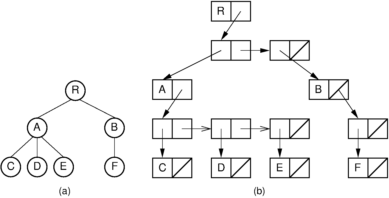
Figure 27.9.5: A dynamic general tree representation with linked lists of child pointers. (a) The general tree. (b) The tree representation.¶

27.9.1.5. Dynamic Left-Child/Right-Sibling Implementation¶

The “left-child/right-sibling” implementation stores a fixed number of pointers with each node. This can be readily adapted to a dynamic implementation. In essence, we substitute a binary tree for a general tree. Each node of the “left-child/right-sibling” implementation points to two “children” in a new binary tree structure. The left child of this new structure is the node’s first child in the general tree. The right child is the node’s right sibling. We can easily extend this conversion to a forest of general trees, because the roots of the trees can be considered siblings. Converting from a forest of general trees to a single binary tree is illustrated by Figure 27.9.6. Here we simply include links from each node to its right sibling and remove links to all children except the leftmost child. Figure 27.9.7 shows how this might look in an implementation with two pointers at each node. Compared with the implementation illustrated by Figure 27.9.5 which requires overhead of three pointers/node, the implementation of Figure 27.9.7 only requires two pointers per node. The representation of Figure 27.9.7 is likely to be easier to implement, space efficient, and more flexible than the other implementations presented in this section.

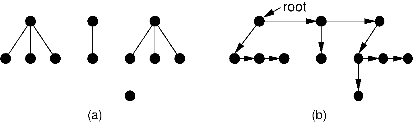
Figure 27.9.6: Converting from a forest of general trees to a single binary tree. Each node stores pointers to its left child and right sibling. The tree roots are assumed to be siblings for the purpose of converting.¶

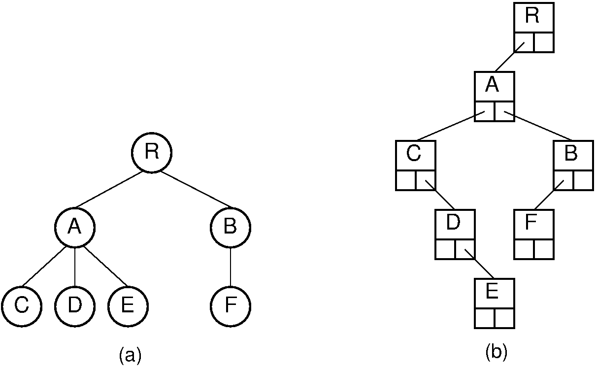
Figure 27.9.7: A general tree converted to the dynamic “left-child/right-sibling” representation. Compared to the representation of Figure 27.9.5, this representation requires less space.¶