10.2.1. Reductions¶

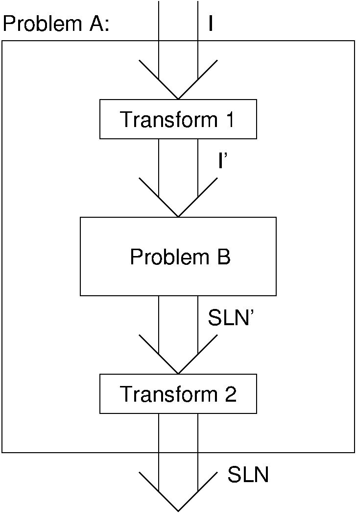
This module introduces an important concept for understanding the relationships between problems, called reduction. Reduction allows us to solve one problem in terms of another. Equally importantly, when we wish to understand the difficulty of a problem, reduction allows us to make relative statements about upper and lower bounds on the cost of a problem (as opposed to an algorithm or program).

Because the concept of a problem is discussed extensively in this chapter, we want notation to simplify problem descriptions. Throughout this chapter, a problem will be defined in terms of a mapping between inputs and outputs, and the name of the problem will be given in all capital letters. Thus, a complete definition of the sorting problem could appear as follows:

1 / 25 Settings

<<<>>>

Here is a visual explanation of the Sorting Problem. We Have:

Input: An unsorted array of records: R1, R2, ..., Rn with associated key values: K1, K2, ..., kn.

1. K10
2. K21
3. K32
4. K43
5. K54
6. K65

Sorting
Algorithm

input

output

1. Ks10
2. Ks21
3. Ks32
4. Ks43
5. Ks54
6. Ks65

1. 4
2. 3
3. 5
4. 1
5. 2
6. 0

1. 0
2. 1
3. 2
4. 3
5. 4
6. 5

23

48

42

59

17

11

93

89

88

12

12

91

57

64

90

34

An illustration of PAIRING. The two lists of numbers are paired up so that the least values from each list make a pair, the next smallest values from each list make a pair, and so on.

In terms of asymptotic notation, assuming that we can find one method to convert the inputs to PAIRING into inputs to SORTING fast enough, and a second method to convert the result of SORTING back to the correct result for PAIRING fast enough, then the asymptotic cost of PAIRING cannot be more than the cost of SORTING.

In this case, there is little work to be done to convert from PAIRING to SORTING, or to convert the answer from SORTING back to the answer for PAIRING, so the dominant cost of this solution is performing the sort operation. Thus, an upper bound for PAIRING is in $O(n \log n)$.

1. 23
2. 42
3. 17
4. 93
5. 88
6. 12
7. 57
8. 90

1. 48
2. 59
3. 11
4. 89
5. 12
6. 91
7. 64
8. 34

Arrays to be paired

1. 23
2. 42
3. 17
4. 93
5. 88
6. 12
7. 57
8. 90

1. 48
2. 59
3. 11
4. 89
5. 12
6. 91
7. 64
8. 34

Transformation - Identity function Cost= O(n)

Reduction is a three-step process. The first step is to convert an instance of PAIRING into two instances of SORTING. The conversion step in this example is not very interesting; it simply takes each sequence and assigns it to an array to be passed to SORTING. The second step is to sort the two arrays (i.e., apply SORTING to each array). The third step is to convert the output of SORTING to the output for PAIRING. This is done by pairing the first elements in the sorted arrays, the second elements, and so on.

Sort

Sort

1. 12
2. 17
3. 23
4. 42
5. 57
6. 88
7. 90
8. 93

Sorted arrays

1. 11
2. 12
3. 34
4. 48
5. 59
6. 64
7. 89
8. 91

Reverse Transformation Cost= O(n)

Paired array

Saving...
Server Error
Resubmit

10.2.1.1. Reduction and Finding a Lower Bound¶

1 / 23 Settings

<<<>>>

Reductions and Lower Bounds

There is another use for reductions aside from applying an old algorithm to solve a new problem (and thereby establishing an upper bound for the new problem). We can use reductions to prove a lower bound on the cost of a new problem by showing that it could be used as a solution for an old problem with a known lower bound.

Problem A:

I

Transfrom 1

Problem B

Transfrom 2

I'

SLN'

SLN

This figure shows a graphical representation of the general reduction process, showing the role of the two problems, and the two transformations.

1. 230
2. 421
3. 172
4. 933
5. 884
6. 125
7. 576
8. 907

Array to be sorted

Transformation (Cost=O(n))

1. 0
2. 1
3. 2
4. 3
5. 4
6. 5
7. 6
8. 7

Position
array

1. 23
2. 42
3. 17
4. 93
5. 88
6. 12
7. 57
8. 90

Input
array

Pairing

1. 0
2. 1
3. 2
4. 3
5. 4
6. 5
7. 6
8. 7

1. 23
2. 42
3. 17
4. 93
5. 88
6. 12
7. 57
8. 90

Pairs generated

1. 23,2
2. 42,3
3. 17,1
4. 93,7
5. 88,5
6. 12,0
7. 57,4
8. 90,6

Reverse Transformation Cost = O(n)

1. 0
2. 1
3. 2
4. 3
5. 4
6. 5
7. 6
8. 7

Saving...
Server Error
Resubmit

Figure 10.2.1: The general process for reduction shown as a “blackbox” diagram.¶

10.2.2. Reduction Examples¶

1 / 23 Settings

<<<>>>

As an example of reduction, consider the simple problem of multiplying two $n$-digit numbers.

1. 0
2. A

1. A^T
2. 0

Here 0 stands for an n×n matrix composed of zero values, A is the original matrix, and AT stands for the transpose of matrix A.

Note that the resulting matrix is now symmetric.

1. 0
2. B^T

1. B
2. 0

=

1. AB
2. 0

1. 0
2. A^TB^T

In the above formula, AB is the result of multiplying matrices A and B together.

1. 2
2. 3

1. 6
2. 7

1. 4
2. 9

X

1. 1
2. 10
3. 5

1. 12
2. 8
3. 11

Transformation (Cost:O(mn))

Transformation (Cost:O(mn))

1. 0
2. 0
3. 0
4. 2
5. 3

1. 0
2. 0
3. 0
4. 6
5. 7

1. 0
2. 0
3. 0
4. 4
5. 9

1. 2
2. 6
3. 4
4. 0
5. 0

1. 3
2. 7
3. 9
4. 0
5. 0

X

1. 0
2. 0
3. 0
4. 1
5. 12

1. 0
2. 0
3. 0
4. 10
5. 8

1. 0
2. 0
3. 0
4. 5
5. 11

1. 1
2. 10
3. 5
4. 0
5. 0

1. 12
2. 8
3. 11
4. 0
5. 0

Multiply

1. 38
2. 44
3. 43
4. 0
5. 0

1. 90
2. 116
3. 107
4. 0
5. 0

1. 112
2. 112
3. 119
4. 0
5. 0

1. 0
2. 0
3. 0
4. 82
5. 116

1. 0
2. 0
3. 0
4. 118
5. 191

Reverse Transform (O(mn))

1. 38
2. 44
3. 43

1. 90
2. 116
3. 107

1. 112
2. 112
3. 119

Output Array

-3

0

2

5

10

1

2

3

9

(-3, $\sqrt{91}$)

(2, $\sqrt{96}$)

(5, $\sqrt{75}$)

Input to SORTING: the values 5, -3, 2, 0, 10. When converted to points, they fall on a circle as shown.

Saving...
Server Error
Resubmit