30.5.1.1. Hashing (1)¶

Hashing: The process of mapping a key value to a position in a table.

A hash function maps key values to positions. It is denoted by $h$.

A hash table is an array that holds the records. It is denoted by HT.

HT has $M$ slots, indexed form 0 to $M-1$.

30.5.1.2. Hashing (2)¶

For any value $K$ in the key range and some hash function $h$, $h(K) = i$, $0 <= i < M$, such that key(HT[i]) $= K$.

Hashing is appropriate only for sets (no duplicates).

Good for both in-memory and disk-based applications.

Answers the question "What record, if any, has key value K?"

30.5.1.3. Simple Examples¶

1 / 10 Settings

<<<>>>

We will demonstrate the simplest hash function, storing records in an array of size 10.

1. 0
2. 1
3. 2
4. 3
5. 4
6. 5
7. 6
8. 7
9. 8
10. 9

Saving...
Server Error
Resubmit

• More reasonable example:

  • Store about 1000 records with keys in range 0 to 16,383.
  • Impractical to keep a hash table with 16,384 slots.
  • We must devise a hash function to map the key range to a smaller table.

30.5.1.4. Collisions (1)¶

• Given: hash function h with keys $k_1$ and $k_2$. $\beta$ is a slot in the hash table.
• If $\mathbf{h}(k_1) = \beta = \mathbf{h}(k_2)$, then $k_1$ and $k_2$ have a collision at $\beta$ under h.

• Search for the record with key $K$:

  1. Compute the table location $\mathbf{h}(K)$.
  2. Starting with slot $\mathbf{h}(K)$, locate the record containing key $K$ using (if necessary) a collision resolution policy.

30.5.1.5. Collisions (2)¶

• Collisions are inevitable in most applications.

  • Example: Among 23 people, some pair is likely to share a birthday.

30.5.1.6. Hash Functions (1)¶

• A hash function MUST return a value within the hash table range.
• To be practical, a hash function SHOULD evenly distribute the records stored among the hash table slots.
• Ideally, the hash function should distribute records with equal probability to all hash table slots. In practice, success depends on distribution of actual records stored.

30.5.1.7. Hash Functions (2)¶

• If we know nothing about the incoming key distribution, evenly distribute the key range over the hash table slots while avoiding obvious opportunities for clustering.
• If we have knowledge of the incoming distribution, use a distribution-dependent hash function.

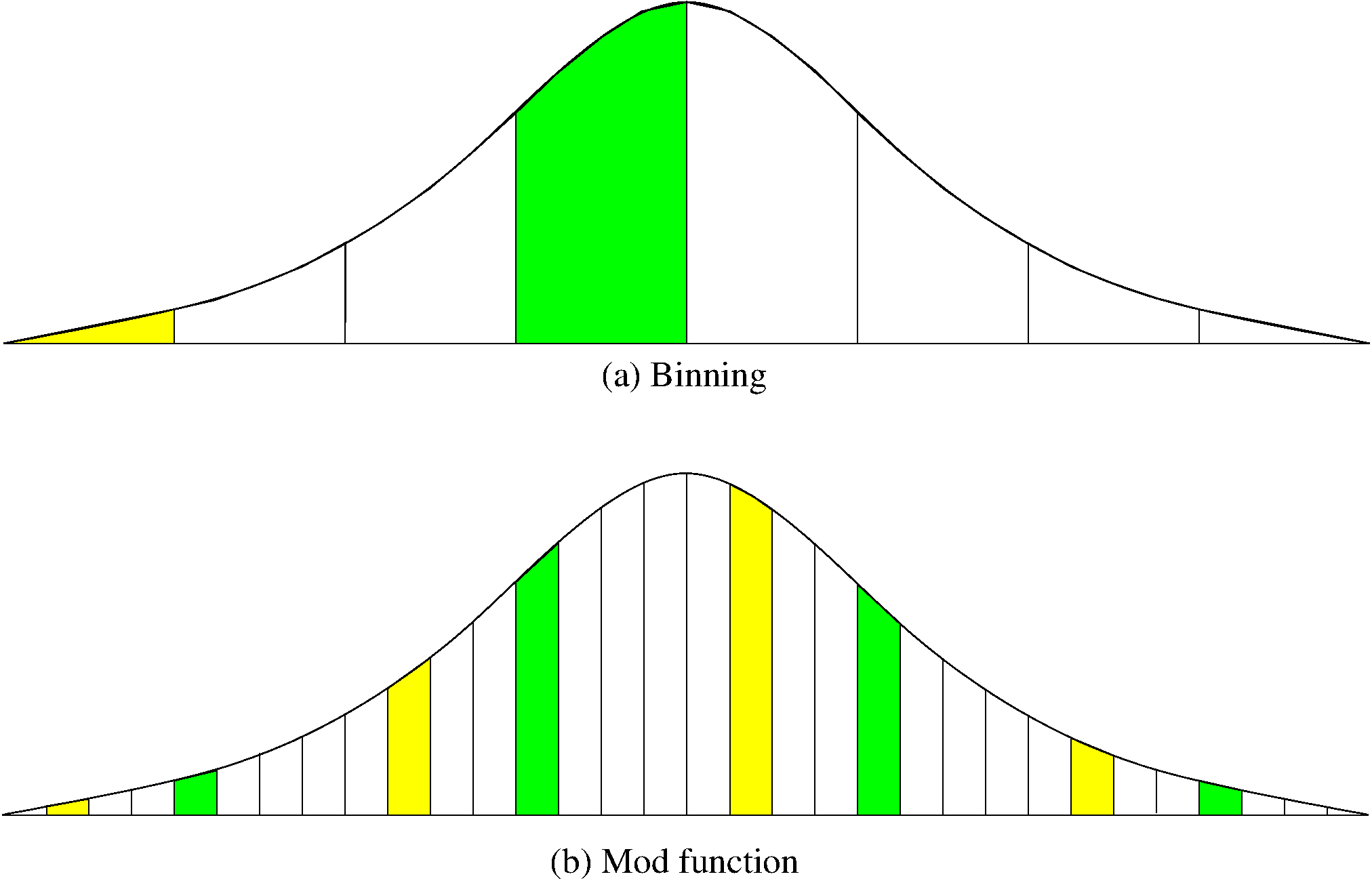
30.5.1.8. Simple Mod Function¶

int h(int x) {
  return x % 16;
}

1 / 10 Settings

<<<>>>

We will demonstrate the mod hash function. To make the compuation easy (because you can probably do mod by 10 in your head easily) we will store records in an array of size 10.

1. 0
2. 1
3. 2
4. 3
5. 4
6. 5
7. 6
8. 7
9. 8
10. 9

Saving...
Server Error
Resubmit

30.5.1.9. Binning¶

1 / 8 Settings

<<<>>>

We will demonstrate the Binning hash function. To make the compuation easy (because you can probably divide by 10 in your head easily) we will store records in an array of size 10.

1. 0
2. 1
3. 2
4. 3
5. 4
6. 5
7. 6
8. 7
9. 8
10. 9

Saving...
Server Error
Resubmit

30.5.1.10. Mod vs. Binning¶

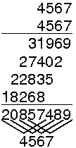
30.5.1.11. Mid-Square Method¶

30.5.1.12. Strings Function: Character Adding¶

int sascii(String x, int M) {
  char ch[];
  ch = x.toCharArray();
  int xlength = x.length();

  int i, sum;
  for (sum=0, i=0; i < x.length(); i++)
    sum += ch[i];
  return sum % M;
}

30.5.1.13. String Folding¶

// Use folding on a string, summed 4 bytes at a time
int sfold(String s, int M) {
  long sum = 0, mul = 1;
  for (int i = 0; i < s.length(); i++) {
    mul = (i % 4 == 0) ? 1 : mul * 256;
    sum += s.charAt(i) * mul;
  }
  return (int)(Math.abs(sum) % M);
}

30.5.1.14. Open Hashing¶

1. 0
2. 1
3. 2
4. 3
5. 4
6. 5
7. 6
8. 7
9. 8
10. 9

100

930

313

977

207

157

979

30.5.1.15. Bucket Hashing (1)¶

1 / 27 Settings

<<<>>>

Demonstration of bucket hash for an array of size 10 storing 5 buckets, each two slots in size. The alternating gray and white cells indicate the buckets.

1. 0
2. 1
3. 2
4. 3
5. 4
6. 5
7. 6
8. 7
9. 8
10. 9

B0

B1

B2

B3

B4

Overflow

Saving...
Server Error
Resubmit

30.5.1.16. Bucket Hashing (2)¶

1 / 21 Settings

<<<>>>

Demonstration of alternative bucket hash for an array of size 10 storing 5 buckets, each two slots in size. The alternating gray and white cells indicate the buckets.

1. 0
2. 1
3. 2
4. 3
5. 4
6. 5
7. 6
8. 7
9. 8
10. 9

B0

B1

B2

B3

B4

Overflow

Saving...
Server Error
Resubmit

30.5.1.17. Closed Hashing¶

• Closed hashing stores all records directly in the hash table.
• Each record $i$ has a home position $\mathbf{h}(k_i)$.
• If another record occupies the home position for $i$, then another slot must be found to store $i$.
• The new slot is found by a collision resolution policy.
• Search must follow the same policy to find records not in their home slots.

30.5.1.18. Collision Resolution¶

• During insertion, the goal of collision resolution is to find a free slot in the table.
• Probe sequence: The series of slots visited during insert/search by following a collision resolution policy.
• Let $\beta_0 = \mathbf{h}(K)$. Let $(\beta_0, \beta_1, ...)$ be the series of slots making up the probe sequence.

30.5.1.19. Insertion¶

// Insert e into hash table HT
void hashInsert(const Key& k, const Elem& e) {
  int home;                     // Home position for e
  int pos = home = h(k);        // Init probe sequence
  for (int i=1; EMPTYKEY != (HT[pos]).key(); i++) {
    pos = (home + p(k, i)) % M; // probe
    if (k == HT[pos].key()) {
      println("Duplicates not allowed");
      return;
    }
  }
  HT[pos] = e;
}

30.5.1.20. Search¶

// Search for the record with Key K
bool hashSearch(const Key& K, Elem& e) const {
  int home;              // Home position for K
  int pos = home = h(K); // Initial position is the home slot
  for (int i = 1;
       (K != (HT[pos]).key()) && (EMPTYKEY != (HT[pos]).key());
       i++)
    pos = (home + p(K, i)) % M; // Next on probe sequence
  if (K == (HT[pos]).key()) {   // Found it
    e = HT[pos];
    return true;
  }
  else return false;            // K not in hash table
}

30.5.1.21. Probe Function¶

• Look carefully at the probe function p():

  pos = (home + p(k, i)) % M; // probe
  

• Each time p() is called, it generates a value to be added to the home position to generate the new slot to be examined.

• $p()$ is a function both of the element's key value, and of the number of steps taken along the probe sequence. Not all probe functions use both parameters.

30.5.1.22. Linear Probing (1)¶

• Use the following probe function:

  p(K, i) = i;
  

• Linear probing simply goes to the next slot in the table.

• Past bottom, wrap around to the top.

• To avoid infinite loop, one slot in the table must always be empty.

30.5.1.23. Linear Probing (2)¶

1 / 11 Settings

<<<>>>

The simplest collsion resolution method is called linear probing. We simply move to the right in the table from the home slot, wrapping around to the beginning if necessary.

1. 0
2. 1
3. 2
4. 3
5. 4
6. 5
7. 6
8. 7
9. 8
10. 9

Saving...
Server Error
Resubmit

30.5.1.24. Problem with Linear Probing¶

1 / 7 Settings

<<<>>>

Consider the situation where we left off in the last slide show. If at this point we wanted to insert the value 3348, we would have to probe all the way to slot 2.

1. 90500
2. 72001
3. 2
4. 3
5. 4
6. 5
7. 6
8. 98777
9. 20378
10. 10599

60%

10%

10%

10%

10%

Saving...
Server Error
Resubmit

• The primary goal of a collision resolution mechanism:

  • Give each empty slot of the table an equal probability of receiving the next record.

30.5.1.25. Linear Probing by Steps (1)¶

• Instead of going to the next slot, skip by some constant c.

  • Warning: Pick M and c carefully.

1 / 10 Settings

<<<>>>

When doing collision resolution with linear probing by steps of size 2 on a hash table of size 10, a record that hashes to slot 4...

1. 0
2. 1
3. 2
4. 3
5. 4
6. 5
7. 6
8. 7
9. 8
10. 9

Saving...
Server Error
Resubmit

• This effectively splits the key range, and the hash table, into two halves. This leads to reduced performance.

30.5.1.26. Linear Probing by Steps (2)¶

• The probe sequence SHOULD cycle through all slots of the table.

  • Pick $c$ to be relatively prime to $M$.

1 / 11 Settings

<<<>>>

When doing collision resolution with linear probing by steps of size 3 on a hash table of size 10, a record that hashes to slot 4...

1. 0
2. 1
3. 2
4. 3
5. 4
6. 5
7. 6
8. 7
9. 8
10. 9

Saving...
Server Error
Resubmit

30.5.1.27. Pseudo-Random Probing (1)¶

1 / 14 Settings

<<<>>>

Let's see an example of collision resolution using pseudorandom probing on a hash table of size 10 using the simple mod hash function.

1. 0
2. 1
3. 2
4. 3
5. 4
6. 5
7. 6
8. 7
9. 8
10. 9

Permutation:

1. 00
2. 31
3. 72
4. 63
5. 14
6. 45
7. 96
8. 27
9. 58
10. 89

Saving...
Server Error
Resubmit

30.5.1.28. Pseudo-Random Probing (2)¶

1 / 11 Settings

<<<>>>

First recall what happens with linear probing by steps of 2. Say that one record hashes to slot 4, and another hashes to slot 6.

1. 0
2. 1
3. 2
4. 3
5. 1044
6. 5
7. 9366
8. 7
9. 8
10. 9

1. 00
2. 31
3. 12
4. 43
5. 94
6. 75
7. 66
8. 27
9. 58
10. 89

Saving...
Server Error
Resubmit

30.5.1.29. Quadratic Probing¶

1 / 3 Settings

<<<>>>

Under quadratic probing, two keys with different home positions will have diverging probe sequences. Consider a value that hashes to slot 5. Its probe sequence is 5, then 5 + 1 = 6, then 5 + 4 = 9, then (5 + 9) % 10 = 4, and so on.

1. 0
2. 1
3. 2
4. 3
5. 4
6. 5
7. 6
8. 7
9. 8
10. 9

Saving...
Server Error
Resubmit

1 / 3 Settings

<<<>>>

Unfortunately, quadratic probing has the disadvantage that typically not all hash table slots will be on the probe sequence.

1. 0
2. 1
3. 2
4. 3
5. 4
6. 5
7. 6
8. 7
9. 8
10. 9

Saving...
Server Error
Resubmit

30.5.1.30. Double Hashing (1)¶

1 / 9 Settings

<<<>>>

Let's see what happens when we use a hash table of size M = 11 (a prime number), our primary hash function is a simple mod on the table size (as usual), and our secondary hash function is h₂(k) = 1 + (k % (M-1)).

1. 0
2. 1
3. 2
4. 3
5. 4
6. 5
7. 6
8. 7
9. 8
10. 9
11. 10

h₂(k) = 1 + (k % (M-1))

Saving...
Server Error
Resubmit

30.5.1.31. Double Hashing (2)¶

1 / 7 Settings

<<<>>>

Now we try the alternate second hash function. Use a hash table of size M = 16 (a power of 2), our primary hash function is a simple mod on the table size (as usual), and our secondary hash function is to do linear probing by steps of size h₂(k) = (((k/M) % (M/2)) * 2) + 1.

1. 0
2. 1
3. 2
4. 3
5. 4
6. 5
7. 6
8. 7
9. 8
10. 9
11. 10
12. 11
13. 12
14. 13
15. 14
16. 15

h₂(k) = (((k/M) % (M/2)) * 2) + 1

Saving...
Server Error
Resubmit

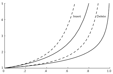
30.5.1.32. Analysis of Closed Hashing¶

The load factor is $\alpha = N/M$ where $N$ is the number of records currently in the table.

30.5.1.33. Deletion¶

• Deleting a record must not hinder later searches.
• We do not want to make positions in the hash table unusable because of deletion.
• Both of these problems can be resolved by placing a special mark in place of the deleted record, called a tombstone.
• A tombstone will not stop a search, but that slot can be used for future insertions.

30.5.1.34. Tombstones (1)¶

1 / 16 Settings

<<<>>>

Let's see an example of the deletion process in action. As usual, our example will use a hash table of size 10, the simple mod hash function, and collision resolution using simple linear probing.

1. 0
2. 1
3. 2
4. 3
5. 4
6. 5
7. 6
8. 7
9. 8
10. 9

Saving...
Server Error
Resubmit

30.5.1.35. Tombstones (2)¶

• Unfortunately, tombstones add to the average path length.

• Solutions:

  1. Local reorganizations to try to shorten the average path length.
  2. Periodically rehash the table (by order of most frequently accessed record).