27.1. The Sparse Matrix¶

Sometimes we need to represent a large, two-dimensional matrix where many of the elements have a value of zero. A difficult situation arises when the vast majority of values stored in an \(n \times m\) matrix are zero, but there is no restriction on which positions are zero and which are non-zero. This is known as a sparse matrix.

One approach to representing a sparse matrix is to concatenate (or otherwise combine) the row and column coordinates into a single value and use this as a key in a hash table. Thus, if we want to know the value of a particular position in the matrix, we search the hash table for the appropriate key. If a value for this position is not found, it is assumed to be zero. This is an ideal approach when all queries to the matrix are in terms of access by specified position. However, if we wish to find the first non-zero element in a given row, or the next non-zero element below the current one in a given column, or recover all of the non-zero values in a given column, then the hash table requires us to check sequentially through the entire table.

Another approach is to implement the matrix as an orthogonal list. Consider the following sparse matrix:

The corresponding orthogonal array is shown in the Figure. Here we have a list of row headers, each of which contains a pointer to a list of matrix records. A second list of column headers also contains pointers to matrix records. Each non-zero matrix element stores pointers to its non-zero neighbors in the row, both following and preceding it. Each non-zero element also stores pointers to its non-zero neighbors following and preceding it in the column. Thus, each non-zero element stores its own value, its position within the matrix, and four pointers. Non-zero elements are found by traversing a row or column list. Note that the first non-zero element in a given row could be in any column; likewise, the neighboring non-zero element in any row or column list could be at any (higher) row or column in the array.

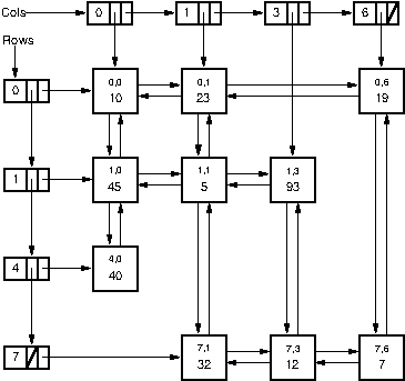
Figure 27.1.1: A representative orthogonal list sparse matrix representation. Depending on the needs of the application, a given cell might store references as part of a singly linked or doubly linked list, and the cell might store row/column positions for the cell or might store references back to the row/column headers.¶

What exactly should be stored in the various (non-zero) cells of the sparse matrix depends on the application. In some cases, knowing the row/column locations for individual cells is important. For example, if we want to normal math operations on matricies, such as add two matricies that are stored using the sparse matrix representation, then it is an important part of each cell comparison to know were exactly we are in the array any natural traversal of the arrays. Thus, each non-zero element would store its row and column position explicitly. To find if a particular position in the matrix contains a non-zero element, we traverse the appropriate row or column list. For example, when looking for the element at Row 7 and Column 1, we can traverse the list either for Row 7 or for Column 1. When traversing a row or column list, if we come to an element with the correct position, then its value is non-zero. If we encounter an element with a higher position, then the element we are looking for is not in the sparse matrix. In this case, the element’s value is zero. For example, when traversing the list for Row 7 in the matrix of the figure, we first reach the element at Row 7 and Column 1. If this is what we are looking for, then the search can stop. If we are looking for the element at Row 7 and Column 2, then the search proceeds along the Row 7 list to next reach the element at Column 3. At this point we know that no element at Row 7 and Column 2 is stored in the sparse matrix.

In some applications, a given row or column represents a vector of information about some object. For example, consider if we want to store a database about reviewer ratings of movies. If there are a lot of movies and a lot of reviewers in the database, then no reviewer will have reviewed a signficant fraction of the movies, and no movie will have been reviewed by a significant fraction of reviewers. So a sparse matrix representation might be ideal, where each column stores the ratings information for a given reviewer, and each row stores the ratings information for a given movie. This allows operations like finding all reviews by a given reviewer However, which column a given movie is in is arbitrary. In this case, each (non-zero) cell of the sparse matrix might need to store a reference to its row and column headers (which might provide further information about the record, such as movie and review information), but the cells probably do not need to store meaningless row/column numbers.

Insertion and deletion can be performed by working in a similar way to insert or delete elements within the appropriate row and column lists.

Each non-zero element stored in the sparse matrix representation takes much more space than an element stored in a simple \(n \times n\) matrix. When is the sparse matrix more space efficient than the standard representation? To calculate this, we need to determine how much space the standard matrix requires, and how much the sparse matrix requires. The size of the sparse matrix depends on the number of non-zero elements (we will refer to this value as NNZ), while the size of the standard matrix representation does not vary. We need to know the (relative) sizes of a pointer and a data value. For simplicity, our calculation will ignore the space taken up by the row and column header (which is not much affected by the number of elements in the sparse array).

As an example, assume that a data value, a row or column index, and a pointer each require four bytes. An \(n \times m\) matrix requires \(4nm\) bytes. The sparse matrix requires 28~bytes per non-zero element (four pointers, two array indices, and one data value). If we set \(X\) to be the percentage of non-zero elements, we can solve for the value of \(X\) below which the sparse matrix representation is more space efficient. Using the equation \(28X = 4mn\) and solving for \(X\), we find that the sparse matrix using this implementation is more space efficient when \(X < 1/7\), that is, when less than about 14% of the elements are non-zero. Different values for the relative sizes of data values, pointers, or matrix indices can lead to a different break-even point for the two implementations.

The time required to process a sparse matrix should ideally depend on NNZ. When searching for an element, the cost is the number of elements preceding the desired element on its row or column list. The cost for operations such as adding two matrices should be \(\Theta(n + m)\) in the worst case when the one matrix stores \(n\) non-zero elements and the other stores \(m\) non-zero elements.

Another representation for sparse matrices is sometimes called the Yale representation. Matlab uses a similar representation, with a primary difference being that the Matlab representation uses column-major order. (Scientific packages tend to prefer column-oriented representations for matrices since this the dominant access need for the operations to be performed.) The Matlab representation stores the sparse matrix using three lists. The first is simply all of the non-zero element values, in column-major order. The second list stores the start position within the first list for each column. The third list stores the row positions for each of the corresponding non-zero values. In the Yale representation, the matrix of the figure above would appear as:

If the matrix has \(c\) columns, then the total space required will be proportional to \(c + 2 NNZ\). This is good in terms of space. It allows fairly quick access to any column, and allows for easy processing of the non-zero values along a column. However, it does not do a good job of providing access to the values along a row, and is terrible when values need to be added or removed from the representation. Fortunately, when doing computations such as adding or multiplying two sparse matrices, the processing of the input matrices and construction of the output matrix can be done reasonably efficiently.