21.6. Growth Rates Review¶

21.6.1. Growth Rates Review¶

Two functions of $n$ have different growth rates if as $n$ goes to infinity their ratio either goes to infinity or goes to zero.

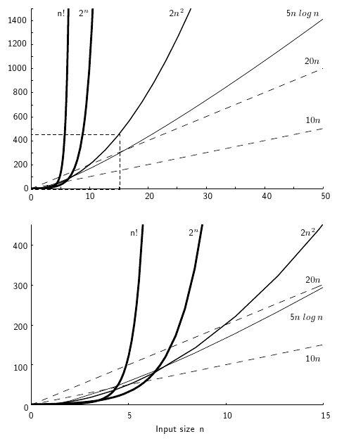
The growth rates for five equations — Figure 21.6.1: Two views of a graph illustrating the growth rates for six equations. The bottom view shows in detail the lower-left portion of the top view. The horizontal axis represents input size. The vertical axis can represent time, space, or any other measure of cost.¶

Where does $(1.618)^n$ go on here?

Exact equations relating program operations to running time require machine-dependent constants. Sometimes, the equation for exact running time is complicated to compute. Usually, we are satisfied with knowing an approximate growth rate.

Example: Given two algorithms with growth rate $c_1n$ and $c_2 2^{n!}$ , do we need to know the values of $c_1$ and $c_2$ ?

Consider $n^2$ and $3n$ . PROVE that $n^2$ must eventually become (and remain) bigger.

Proof by Contradiction: Assume there are some values for constants $r$ and $s$ such that, for all values of $n$ , $n^2 < rn + s$ . Then, $n < r + s/n$ . But, as $n$ grows, what happens to $s/n$ ? It goes to zero.

Since $n$ grows toward infinity, the assumption must be false. Conclusion: In the limit, as $n \rightarrow \infty$ , constants don’t matter. Limits are the typical way to prove that one function grows faster than another.

Here are some useful observatios.

Since $n^2$ grows faster than $n$ ,

$2^{n^2}$ grows faster than $2^n$ . (Take antilog of both sides.)
$n^4$ grows faster than $n^2$ . (Square boths sides.)
$n$ grows faster than $\sqrt{n}$ . ( $n = (\sqrt{n})^2$ . Replace $n$ with $\sqrt{n}$ .)
$2 \log n$ grows no slower than $\log n$ . (Take $\log$ of both sides. Log “flattens” growth rates.)

Since $n!$ grows faster than $2^n$ ,

$n!!$ grows faster than $2^n!$ . (Apply factorial to both sides.)
$2^{n!}$ grows faster than $2^{2^n}$ . (Take antilog of both sides.)
$n!^2$ grows faster than $2^{2n}$ . (Square both sides.)
$\sqrt{n!}$ grows faster than $\sqrt{2^n}$ . (Take square root of both sides.)
$\log n!$ grows no slower than $n$ . (Take log of both sides. Actually, it grows faster since $\log n! = \Theta(n \log n)$ .)

If $f$ grows faster than $g$ , then must $\sqrt{f}$ grow faster than $\sqrt{g}$ ? Yes.

Must $\log f$ grow faster than $\log g$ ? No. $\log n \approx \log n^2$ within a constant factor, that is, the growth rate is the same!

$\log n$ is related to $n$ in exactly the same way that $n$ is related to $2^n$ .

$2^{\log n} = n$ .

21.6.1.1. Asymptotic Notation¶

$\begin{split}\begin{array}{llcl} \mathrm{little\ oh}&f(n) \in o(g(n))&<&\lim f(n)/g(n) = 0\\ \mathrm{big\ oh}&f(n) \in O(g(n))&\leq\\ \mathrm{Theta}&f(n) = \Theta(g(n))&=&f=O(g) and\\ &&& g=O(f)\\ \mathrm{Big\ Omega}&f(n) \in \Omega(g(n))&\geq\\ \mathrm{Little Omega}&f(n) \in \omega(g(n))&>&\lim g(n)/f(n) = 0 \end{array}\end{split}$

I prefer “ $f \in O(n^2)$ ” to “ $f = O(n^2)$ ” While $n \in O(n^2)$ and $n^2 \in O(n^2)$ , $O(n) \neq O(n^2)$ .

Note: Big oh does not say how good an algorithm is—only how bad it can be.

If $\mathcal{A}\in O(n)$ and $\mathcal{B} \in O(n^2)$ , is $\mathcal{A}$ better than $\mathcal{B}$ ? Perhaps… but perhaps better analysis will show that $\mathcal{A} = \Theta(n)$ while $\mathcal{B} = \Theta(\log n)$ .

Order Notation has practical limits. Notation: $\log n^2 (= 2 \log n)$ vs. $\log^2 n (= (\log n)^2)$ vs. $\log \log n$ .

$\log 16^2 = 2 \log 16 = 8$ .

$\log^2 16 = 4^2 = 16$ .

$\log \log 16 = \log 4 = 2$ .

Statement: Resource requirements for Algorithm $\mathcal{A}$ grow slower than resource requirements for Algorithm $\mathcal{B}$ .

Is $\mathcal{A}$ better than $\mathcal{B}$ ?

Potential problems:

How big must the input be?
Some growth rate differences are trivial Example: $\Theta(\log^2 n)$ vs. $\Theta(n^{1/10})$ . If $n$ is $10^{12} (\approx 2^{40})$ then $\log^2 n \approx 1600$ , $n^{1/10} = 16$ even though $n^{1/10}$ grows faster than $\log^2 n$ . $n$ must be enormous (like $2^{150}$ ) for $n^{1/10}$ to be bigger than $\log^2 n$ .

It is not always practical to reduce an algorithm’s growth rate “Practical” here means that the constants might become too much higher when we shave off the minor asymptotic growth.

Shaving a factor of $n$ reduces cost by a factor of a million for input size of a million. Shaving a factor of $\log \log n$ saves only a factor of 4-5.

There is the concept of a “Practicality Window”. In general, (1) we have limited time to solve a problem, and (2) input can only get so big before the computer chokes. Fortunately, algorithm growth rates are USUALLY well behaved, so that Order Notation gives practical indications. “Practical” is the keyword. We use asymptotics because they provide a simple model that usually mirrors reality. This is useful to simplify our thinking.

OpenDSA Data Structures and Algorithms Modules Collection

Chapter 21 Senior Algorithms Course

21.6. Growth Rates Review¶

21.6.1. Growth Rates Review¶

21.6.1.1. Asymptotic Notation¶